Nine methods.
One exact clock.
Loops solved as one.
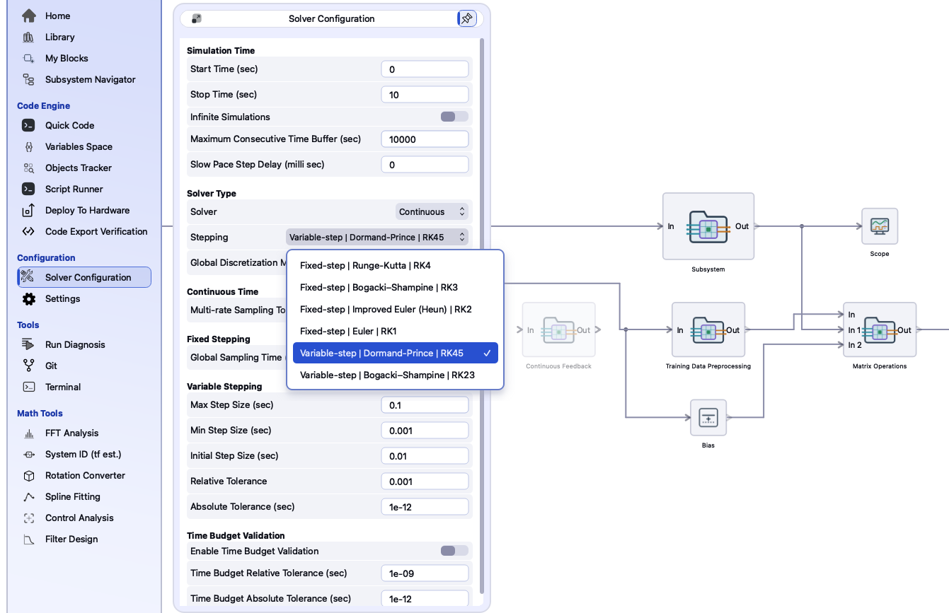
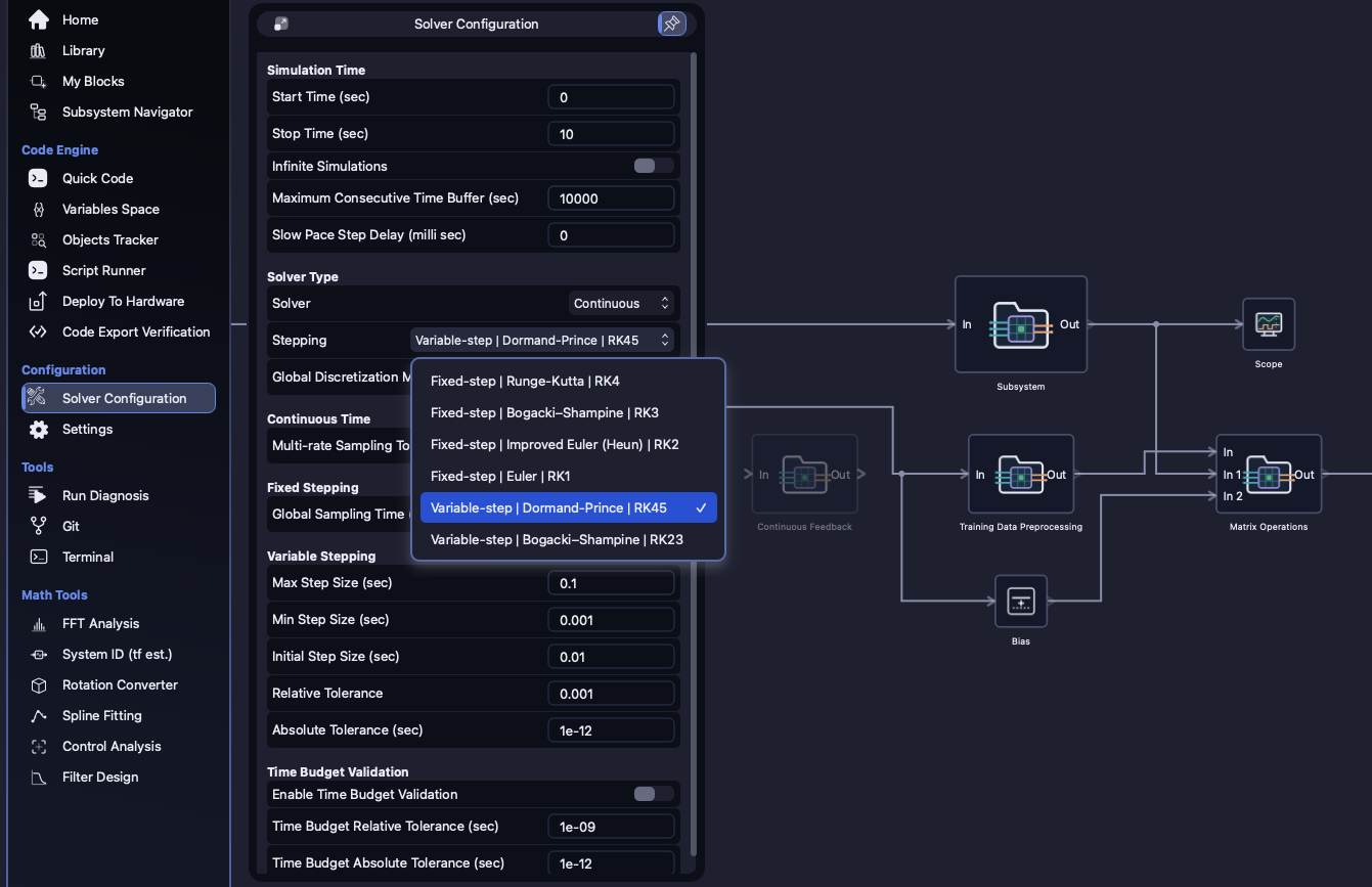
Choose a solver type and one of nine integration methods for the whole model, and let any subsystem keep a rate of its own. Every rate is stepped on one exact grid, and a feedback loop between continuous blocks is integrated as a single system rather than block by block.
Every rate, on one exact clock.
A controller can run slower than the plant it drives, and a subsystem can keep a rate that has nothing to do with the global one. The simulator doesn't let the rates drift apart. It finds the one fine step they all share and steps each block only on its own beats.
This is the worked example from the manual. Each rate is rounded to a multiple of the multi-rate tolerance. The greatest common divisor of those multiples is the fine step, and their least common multiple is the window. The clock advances one window at a time. Inside a window, the Gain is solved at sub-steps 0 and 3 and everything else at 0, 2 and 4. A rate doesn't have to divide the global one; it only has to be a clean multiple of the tolerance.
- Time is a gridThe fixed-step clock is
start + n × Ts, nevert += Ts. So the tenth step ofTs = 0.1lands on exactly 1.0, and a Step set to switch at 1.0 switches on sample 10. Exported code computes its clock the same way. - Rates flow downA block's
Sampling Time (s)defaults to-1, which means it inherits its rate. Home takes the global sampling time, and a subsystem takes its own rate if it sets one and its parent's otherwise. The enclosing level decides a block's rate, not whichever block happens to feed it. - First and lastIn every solver mode, the first sample is
the initial condition and the last is
stopTimeitself. Ten seconds at 0.1 s is 101 samples,t = 0 … 10.
Fixed when you ship. Variable when you study.
A model is Continuous or Discrete. The type says how the model advances,
not what is in it. Most real models are mixed, with continuous dynamics and discrete logic in one
diagram, and that is expected rather than a compromise. Under Continuous, one of nine
methods integrates the continuous parts.
The Runge–Kutta family
Steps at the global sampling time. Fixed-step is what code export needs, because a generated core advances by a known step.
For stiff models you still want to ship
When a model mixes very fast and very slow dynamics and stays stable only at a tiny step, these keep the same sampling time and remain exportable.
The step the dynamics deserve
They choose their own step as they go, within the step bounds and tolerances you set. The step is shortened to land exactly on the moments a source announces in advance: a Step's step time, a pulse edge, a table breakpoint. Those jumps stay sharp instead of being smeared across a step.
The stiff one
The method to try when RK45 crawls or warns that it hit the minimum step size.
Under joint coupling, its Newton iteration runs over the whole state vector at once.
When a continuous description has to run sampled, the Global Discretization Method decides how. It defaults to Zero-order Hold.
A loop is integrated as one system.
Under the Continuous solver, every block's continuous states are gathered
into one state vector and advanced together by the chosen method. The whole diagram is
re-evaluated at every intermediate stage, feedback included. So a loop through integrators,
transfer functions and state spaces has no hidden delay, whatever order the blocks were
created in.
- ExplicitA loop between continuous blocks gets the accuracy of the method you chose, not the accuracy of a one-stage-stale edge.
- ImplicitUnder
TRBDF2, a stiff loop is implicit as a loop, so it settles in a few dozen steps. - Per-blockIt stays selectable. It is the scheme the exported code reproduces, so it is the one to compare a feedback diagram against its export.
Joint:     20 rows; max |x| = 1;     x(0.5) = -2e-16
Per-block:  8 rows; max |x| = 6.7e9;  x(0.5) = -6.7e9
One panel. Or one line.
Everything a run obeys is in Solver Configuration, and every field has a
console equivalent: modelConfig, getModelConfig and
setModelConfig. A study that sweeps solver settings is a script, not an afternoon
of clicking.
setModelConfig solverType: no option matches 'Banana' - available:
  Continuous
  Discrete
getModelConfig and setModelConfig.solverType Continuous steppingType Fixed-step | Runge-Kutta | RK4 solverCoupling Joint | continuous states integrated together discretizationMethod Zero-order Hold multiRateTolerance 1e-09 globalSamplingTime 0.1 maxTimeStep 0.1 minTimeStep 0.001 relativeTolerance 0.001 absoluteTolerance 1e-12
The live solver, against Simulink's.
A pre-release suite puts the solver itself up against Simulink. There are 26 cases. Eight continuous methods each run feedback loops closed through an Integrator, a State Space and a Transfer Function. The Discrete solver runs a discrete-only chain, and RK4 also runs an algebraic loop. TR2 is not a case, because Simulink has no matching solver. Each case builds one diagram and runs it in ICore and in Simulink, under the solver the Simulink bridge maps it to. It checks two things: that the solver settings reached Simulink, and that the two trajectories agree within the tolerance below. For the algebraic loop, both tools have to refuse to run it.
- 1e-9RK1, RK2, RK4, Discrete against
ode1,ode2,ode4andFixedStepDiscrete: the same tableau and the same arithmetic. BE1 againstode1beat 1e-7, since its Newton iteration stops at 1e-10. - 1e-4RK3 against
ode3. Both are third-order, but the tableaus differ (Kutta and Bogacki–Shampine). - 5e-4RK45, RK23 against
ode45andode23. Each side uses its own step controller, with the same 1e-6 relative tolerance. - 2e-3TRBDF2 against
ode23tb: the same method, with different controllers.
What the solver will not do.
- Export a variable stepCode export runs under a fixed-step or discrete solver only, and an exported subsystem needs one rate throughout. A mismatch fails with a list of every block at a different rate.
- Solve algebraic loopsA loop in which every block feeds its input straight through to its output is refused before the run, with the loop named. Break it with a Unit Delay, a Memory, an Integrator or an Algebraic Constraint block.
- Discrete-delay loopsA loop closed through a discrete delay block reads that delay one sample later than Simulink does. It is documented, reproducible behaviour, and the exported code matches ICore's own trajectory.
- Joint across ratesJoint coupling applies to variable step and single-rate fixed step. A multi-rate model keeps the per-block scheme, because its blocks do not step together.
- Locate switchesVariable step lands on discontinuities a source announces in advance. A switch that depends on the signal, such as a Saturation or a Relay, is not located inside a step.
- MatchedThe Matched discretization currently computes the same matrices as Zero-order Hold. The name is reserved.
The equations behind every method are public: Running a simulation · Sample time and loops · Solver mathematics
See also: One model, every rate, every target · Code export
See it run on your own model.
Download the application from the customer portal, or read the documentation first - the manual, a page for every block, and the full command reference are public.