# Matrix of Double
Matrix
The workhorse: arithmetic, decompositions, reductions over all entries or along an axis, and the linear-algebra solvers.
>>> [4 -2; 1 3] \ [1; 2]
[[0.5], [0.5]]
One module holds every number the product computes: the types, the control-systems tooling, the solvers' linear algebra, and the evaluator the console runs on. It is built to give MATLAB's answers, including the ones people don't expect, and those answers were measured against MATLAB rather than assumed.
>>> -2^2-4 # Integer^ binds tighter than unary minus. The precedence table is MATLAB's.
>>> ~1 + 11 # Integer~ is a unary operator, so this reads as (~1) + 1.
>>> numel(0:0.1:1)11 # IntegerEleven, not ten. The colon count follows MATLAB's floating-point rule, and the range ends on 1 exactly.
>>> round(1.005, 2)1.01 # DoubleIt rounds the decimal you typed, not the double just below it.
>>> sind(180)0 # IntegerAn exact zero, where sin(pi) gives 1.22465e-16. No multiple of 90° ever reaches the radian routine.
>>> (-8)^(1/3)1 + 1.73205i # ComplexThe principal root. The answer leaves the real line where MATLAB's does.
>>> sqrtm([1 1; 0 1])[[1, 0.5], [0, 1]] # Matrix of DoubleSchur-based, so it is exact on a defective matrix, where an eigenvector-based root would return noise.
>>> inv([1 2; 2 4])[[Inf, Inf], [Inf, Inf]] # Matrix of DoubleA singular matrix gives MATLAB's answer, not a plausible-looking number.
>>> a = 2; f = @(x) a*x; a = 5; f(3)6 # IntegerA handle captures by value at the moment it is made, the way MATLAB's does.
>>> syms x; expand((x+1)^3)3*x + 3*x^2 + x^3 + 1 # SymExact symbolic algebra, printed in MATLAB's order as well.
Every line above is a
real headless run, ICoreBlocks --console "<line>", copied from its output
with the kind tag the console prints. Each is a case where the obvious implementation gives a
different number from MATLAB. These rules were measured against MATLAB R2026a and written
down, not guessed.
The console prints the kind of every answer, and each kind is a real type in this module, not a display format applied to a matrix. A transfer function stays a transfer function through every operation.
The workhorse: arithmetic, decompositions, reductions over all entries or along an axis, and the linear-algebra solvers.
>>> [4 -2; 1 3] \ [1; 2] [[0.5], [0.5]]
For the places where the answer is not real. Square roots, logs and fractional powers promote to complex exactly where MATLAB's do.
>>> (-8)^(1/3)
1 + 1.73205i
Roots and fitting. A spline's degree is lowered automatically when there are too few points to support it.
>>> polynomial([1 2 3])
x^2 + 2x + 3
A signal with its own time base. This is what a run, or a step, hands back.
>>> y = step(tf([1],[1 1]), 5, 6)
Time Series (6 samples, t = 0 .. 5)
Built with MATLAB's constructors and displayed the way MATLAB displays them, including
tf('s'), which is an improper model.
>>> s = tf('s');
>>> G = 1/(s+1)
G =
    1
  -----
  s + 1
The zeros, poles and gain are kept as themselves. The fraction is worked out only when asked for, so the factored model and the fraction always give the same numbers.
>>> zpk([], [-1 -2], 1)
       1
  -----------
  (s+1) (s+2)
The console's own computer-algebra engine: an expression tree with exact rational arithmetic. There is no third-party CAS underneath.
>>> syms x; int(x^2)
x^3/3
The same text in MATLAB and in the console, so it crosses the MATLAB bridge as it stands.
>>> f = @(x) x.^2
f = @(x) x.^2
The same objects a block holds are the ones you type. Block reduction, the solver and the analysis tools all call into this module.
c2d, d2c and
d2d with zoh, foh, tustin and
impulse. d2c inverts a zero-order hold with a matrix logarithm,
so a plant with a pole at the origin comes back as it was.zpk.step, impulse,
initial and lsim, with samples spaced by MATLAB's own
time-grid rule.bode, margin,
rlocus, pole, dcgain. Design with place,
lqr and pidtune.0.004679 z + 0.004377 --------------------- z^2 - 1.81 z + 0.8187 Sample time: 0.1 seconds Discrete-time transfer function.
    1
  -----
  s + 2
Continuous-time transfer function.
1/(s+1). The closed-loop
pole moves from −1 to −2.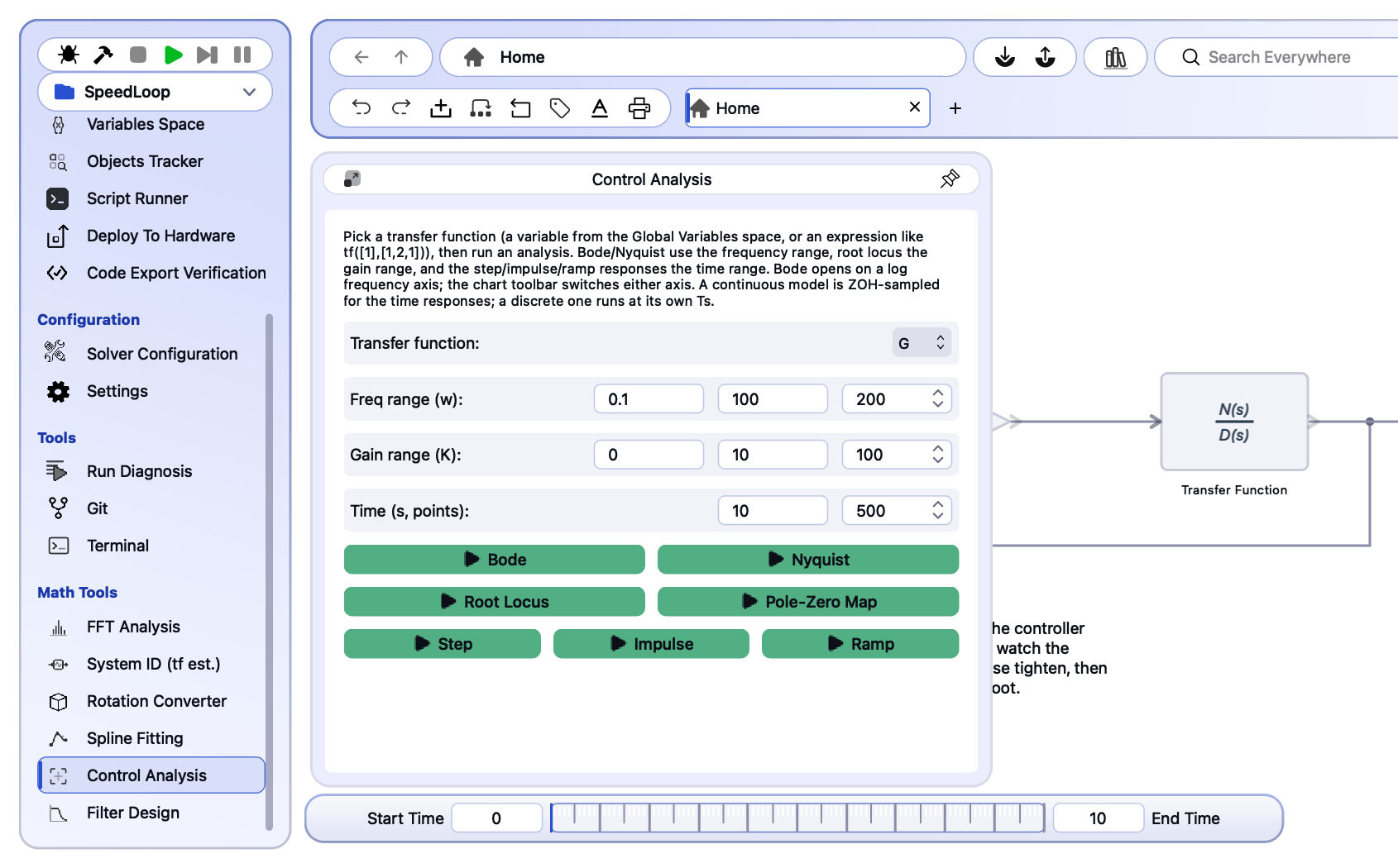
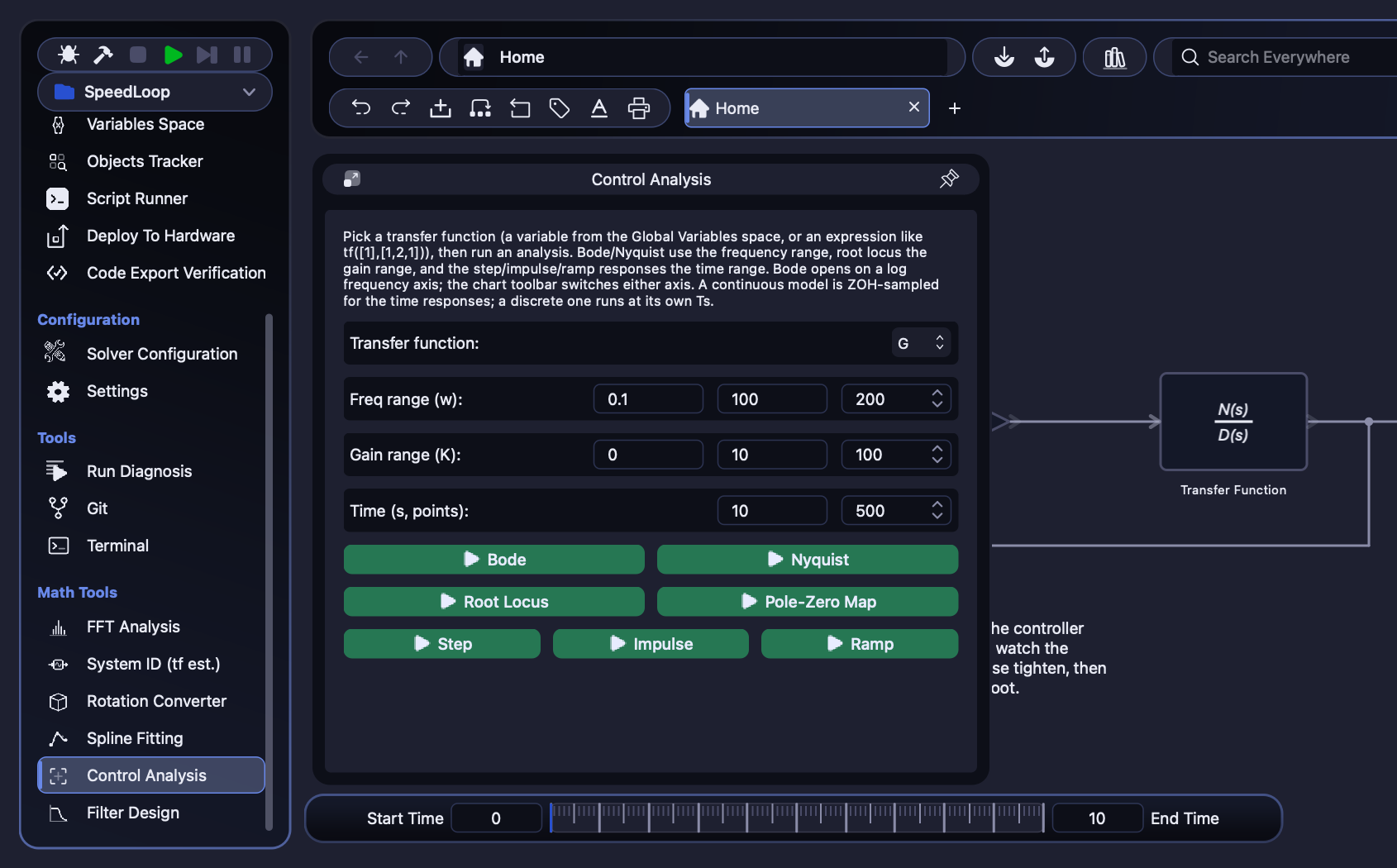
G = tf([1],[1 2 1]) declared in the console, then read straight out of the variables space by the analysis tool - magnitude falling at 40 dB per decade and phase settling at −π, as a double pole at s = −1 should.Calculus, optimization, signal processing, statistics, curve fitting and aerospace sit beside the core. Many of them are transcribed from the MATLAB routine they answer for, rather than approximated by a general-purpose one.
integral(@(x) x.^2, 0, 1) gives 0.333333, with MATLAB's adaptive
Gauss–Kronrod rule behind it.
integralode45trapzexpmint(1/(x^2 + 3*x + 2)) gives log(x + 1) - log(x + 2). The partial
fractions are exact, so the answer isn't a numerical fit.
diffintfactorlaplaceFFTs, digital filter design, zero-phase filtering and spectral estimates. The FFT backend is bundled, so there is no external dependency.
fftbutterfiltfiltpwelchHypothesis tests that keep MATLAB's distinctions, such as ttest(x, y) being
paired and ttest2 being unpaired, so the p-value is the one you meant.
ttestttest2anova1histcountsLinear and quadratic programmes, and fminsearch, which rounds each step
where MATLAB rounds so the two stay together to the last digit.
linprogquadprogfminsearchPolynomial fits, spline and pchip sharing one evaluator, and
MATLAB's linear interp1 as the default.
polyfitinterp1splinepchipThese are not scattered helpers collected under one heading. The console, the solver, the block library and the code generators all compute through ICoreMath. That is why they agree about what a matrix is and what an operation means, and why an expression you can type into the console is one the SDK can evaluate.
When the right answer isn't available, the console refuses and gives the reason, rather than returning a number that looks right and isn't.
c2d(sys, Ts, "matched")
is refused, because the routine under that name was a zero-order hold, and returning one under
MATLAB's name would be wrong in a way nothing on screen shows. Use zoh,
foh, tustin or impulse.{1, 2} and strsplit are refused by
name.rng(seed) makes a run
repeatable, but its stream is not MATLAB's, so the same seed draws different numbers from
MATLAB.schur's eigenvalue order, the difference is recorded rather than hidden.collect. The value is the
same; only the order of the terms differs.The details are in the manual: the core MATLAB catalog · control systems · symbolic math · what the solver will and will not do
See also: Eigen, wrapped · Python and MATLAB, both · MATLAB and Simulink, both ways
Download the application from the customer portal, or read the documentation first - the manual, a page for every block, and the full command reference are public.